Software Management¶

In general, users are encouraged to install and manage their own software and environments on their user space in the sciCORE cluster. For some use cases, however, pre-installed software is available through a module system.

Module System¶

Pre-installed software is made available through a framework called environment modules. By default, no module is loaded when you log in, but the module commands can easily be added to your .bashrc or .bash_profile to automatically load frequently used programs after login.

We have 3 major software stacks available in the sciCORE HPC Cluster:

1. sciCORE EasyBuild

   • This software stack is loaded by default.
   • Activation Command: enable-software-stack-scicore

2. Compute Canada 2023

   • Compute Canada provides a software stack tailored for high-performance computing (HPC) applications. Here is the link to its detailed documentation.
   • Activation Command: enable-software-stack-compute-canada

3. EESSI 2023.06

   • EESSI stands for European Environment for Scientific Software Installations. The EESSI software stack is designed to facilitate collaboration and software deployment across European research institutions. Here is the official link to the documentation.
   • Activation Command: enable-software-stack-eessi

Using the Module System¶

To view the list of available software modules, use:

module av

To see available versions of a specific software package, use

ml spider <softwareName>

Finally, to load a specific software module, run:

ml <softwareName/version-toolchain>

For example, to load the R module version 4.4.2 built with the foss-2024a toolchain, you would run:

ml R/4.4.2-foss-2024a

Strictly speaking, running ml R will also load some version of the R software. However, we recommend to always include the version and toolchain (when applicable) in the module load command for clarity and reproducibility.

enable-software-stack-compute-canada  # Activate Compute Canada stack
ml av  # List available modules in the Compute Canada stack
enable-software-stack-scicore  # Switch back to sciCORE EasyBuild stack
ml av  # List available modules in the sciCORE EasyBuild stack

Module command reference¶

The key module commands are:

• module avail (or ml av): list available modules

• module load <softwareName> (or ml load <softwareName>): load the module <softwareName>

• module list (or ml list): list currently loaded modules

• module spider <keyword> (or ml spider <keyword>): search for modules with keyword in their name or description

• module help (or ml help): list other module commands

• module unload <softwareName> (or ml -<softwareName>): unload the module <softwareName>

• module purge (or ml purge): unload all loaded modules

Python Environment¶

When working with Python software, we recommend creating virtual environments either on a per project basis or for specific package collections that get reused in different contexts. This allows you to avoid conflicts between different Python packages and versions and helps the reproducibility of your work.

In the sciCORE cluster you can manage your virtual environments much like you would on your local machine. You can choose your favorite package manager, be it conda, mamba, uv, pixi, etc.

An environment for a specific research project¶

Let us say you are working on a research project called my_project and you want to write some Python code for it. Let us create a new directory for it and include a single Python script called my_script.py:

mkdir my_project
cd my_project

If you have conda or mamba installed, you can proceed as follows:

conda create -n my_project python=3.10  # or some other version
conda activate my_project
pip install <package_name>  # install packages you need
python my_script.py  # run your scripts within the environment

If you have uv installed, you can create a virtual environment like this:

uv init
uv add <package_name>  # install packages you need
uv run python my_script.py  # run your scripts within the environment

Environments for specific package collections¶

Some environment managers, such as conda or pixi allow you to create environments that are “globally visible”. These are intended to contain tool sets that you could use for general purposes, such as quick data exploration or analysis, or for specific tasks that you perform frequently across different projects.

Any conda environment you create behaves like this by default, because you can activate it from anywhere in the machine. For example, you can create an environment called data_analysis like this:

conda create -n data_analysis python=3.10  # or some other version
conda activate data_analysis
pip install pandas numpy matplotlib ipython  # install packages you need

Then whenever you activate the data_analysis environment, you have access to pandas, numpy, and matplotlib in your Python scripts, no matter where you are in the file system.

For pixi, the syntax to reach a similar result is:

pixi global install --environment data_analysis --expose jupyter --expose ipython jupyter numpy pandas matplotlib ipython

Make sure to check if your package manager supports a feature like this.

Particulars of Jupyter notebooks on Open OnDemand¶

Because Jupyter on Open OnDemand (OOD) is launched from a central process, it does not automatically see the kernels from the Python environments you create. So you need to make sure to follow these steps:

1. Install the ipykernel package in your Python environment¶

With conda or mamba, you can do this by running:

conda activate my_project  # or the name of your environment
conda install ipykernel  # or pip install ipykernel

With uv or pixi:

uv add ipykernel  # or pixi add ipykernel

2. (Not necessary for conda or mamba environments) Register the kernel with Jupyter¶

If your environment manager installs the ipykernel package in a .venv folder within the project’s directory, you need to manually register this kernel with Jupyter.

For example, if you are using uv, navigate to your project directory and run:

uv run python -m ipykernel install --user --name=<project_name> --display-name "Python [uv env: <project_name>]"

where <project_name> is the name of your project.

If you open a new Jupyter notebook on OOD you should now be able to see

"Python [uv env: <project_name>]"

as an option in the kernel selection menu in the top right corner of the notebook interface.

R Environment¶

R is available on the cluster and can be loaded via the module system. You can explore all available R versions with

ml spider R

To load a specific version of R, use the following pattern:

ml R/<version>

For example, to load R/4.3.2-foss-2023a, you would use:

ml R/4.3.2-foss-2023a

After loading the module, you can check that the R executable is available by running:

which R

R scripts in SLURM jobs¶

To run R scripts from inside a SLURM job, the best method is to use the Rscript binary. For example:

#!/bin/bash
#SBATCH ... slurm parameters

module load R/4.3.2-foss-2023a

Rscript myscript.R

You should specify within your R script whether you want to save any files or the workspace. Print statements are directed to STDOUT.

Parallelism in R¶

Some R libraries implement functions that can make use of parallelism to accelerate calculations. The default behavior of these functions is library-specific, with some libraries assuming by default that all the resources on the machine (i.e. all CPUs) can be used by the library. This is a poor design choice which is unfortunately fairly common in the R ecosystem.

When an R script makes use of parallelism in functions, it is the responsibility of the user to verify that the number of cores used by R corresponds to the number of cores reserved with the SLURM script submission. Some users have crashed compute nodes on the cluster because they didn’t understand the behavior of the program they were using. R functions will often have an option that allows specifying the number of cores to use. This can be matched with the variable $SLURM_CPUS_PER_TASK

There are several approaches to parallelism in R. We recommend the use of the packages parallel and foreach. One can also submit R jobs to the cluster using rslurm.

RStudio Server¶

Users can run R code interactively on RStudio Server, which is available as an app on Open OnDemand. See “Interactive Computing” for more information on interactive computing on sciCORE.

Installing R Packages¶

All sciCORE users have the ability to download and install their own R packages. This works in the same way whether using R from the RStudio Server or from a shell session.

You can determine the path for installed packages using the .libPaths() function in R. Common packages maintained by the system administrators are normally installed along with the software build (e.g. /scicore/soft/apps/R/3.6.0-foss-2018b/lib64/R/library) whereas user-installed packages end up in the home folder (e.g. /scicore/home/<groupid>/<userid>/R/x86_64-pc-linux-gnu-library/3.6).

There are various methods for installing R packages, which depend on the code itself and the repository where it lives. Normally, CRAN is the main source to install packages, using the

install.packages()

function. Bioconductor packages are installed using the

BiocManager::install()

function. If you have any questions about installing R packages or run into problems during compilation, please contact us via our Help Center.

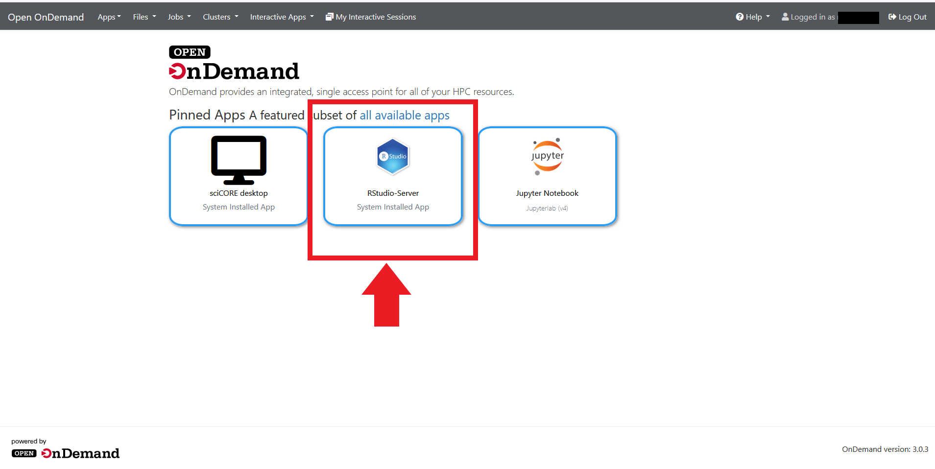
Shiny Apps on R-Studio¶

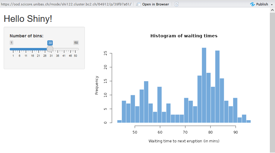
Shiny is a web application framework for R that enables you to turn your analyses into interactive web applications without requiring HTML, CSS, or JavaScript knowledge. Shiny apps can be built using R Studio, an integrated development environment (IDE) for R. Within sciCORE you need to use Open OnDemand (OOD) to connect to the R studio server and run Shiny Apps. The Shiny Apps are by default placed in the ShinyApps/ folder by the user.

These are the steps to use Shiny Apps:

1. Connect to Open On Demand (OOD)¶

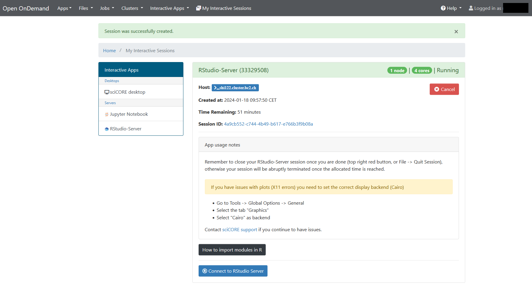
2. Start the R-Studio Server¶

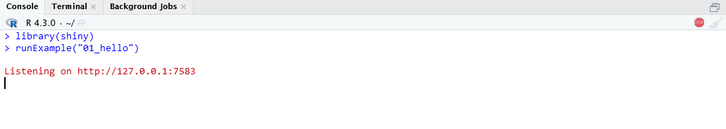
3. Load the Shiny library¶

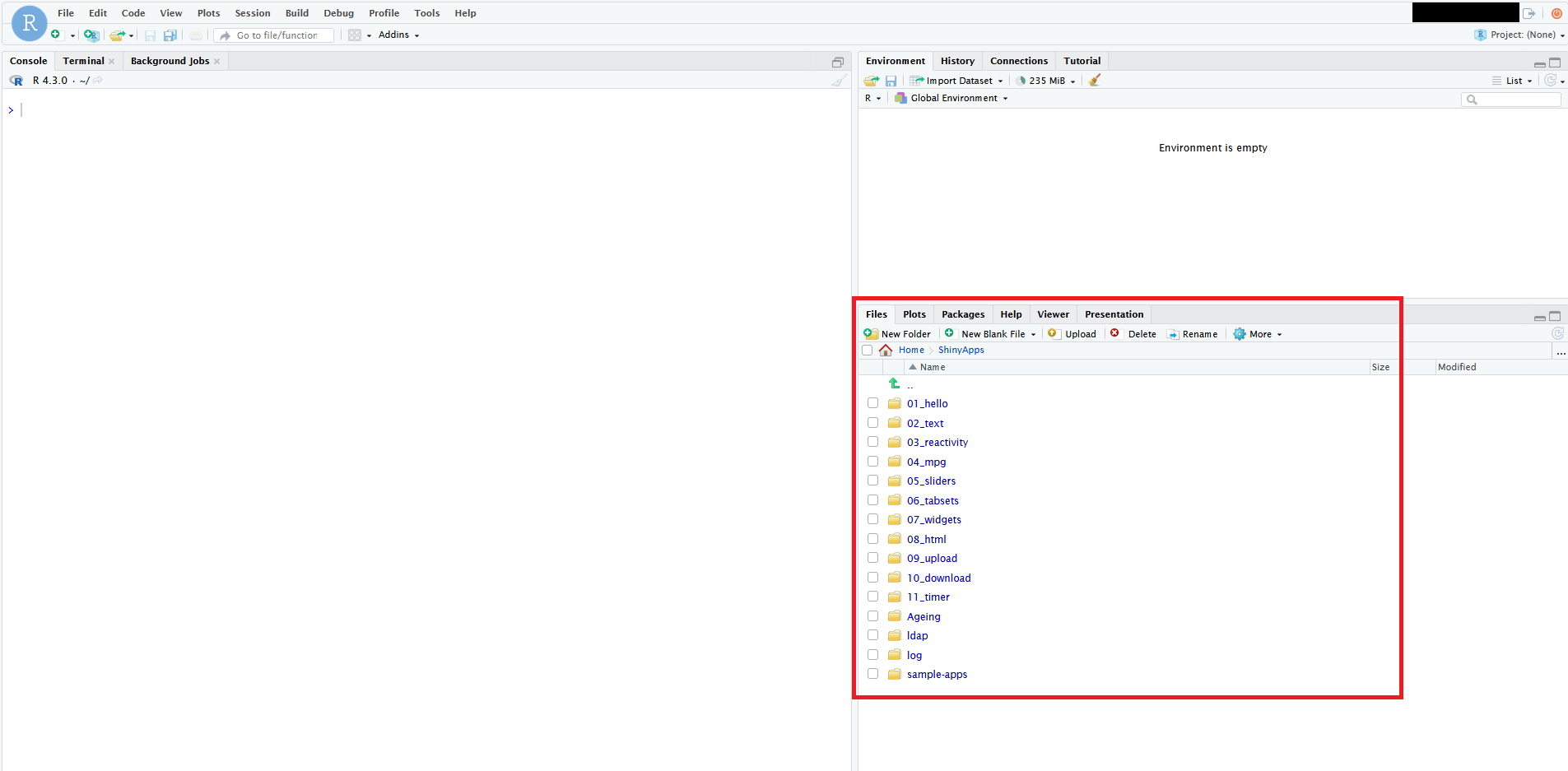
4. Run the available Shiny Apps from their folders¶

runExample("04_mpg/")

runApp("~/ShinyApps/04_mpg/")

MATLAB¶

Interactively¶

To run MATLAB interactively, we recommend opening a sciCORE Desktop session on Open OnDemand.

From within the sciCORE Desktop session, MATLAB can be loaded via the module system. Open a terminal, then type the following to explore all available MATLAB versions with

ml spider MATLAB

To load a specific version of MATLAB, use the following pattern:

ml MATLAB/<version>

For example, to load MATLAB 2023b, you would use:

ml MATLAB/2023b

To run MATLAB with a graphical user interface (GUI) run the following from the command line:

matlab

To have a command-line interface (CLI) with Java Virtual Machine (JVM):

matlab -nodesktop

To run MATLAB without a without JVM, you can use:

matlab -nojvm

In SLURM batch jobs¶

You can submit MATLAB scripts to the computing nodes of the cluster as a regular SLURM job. You only need to take care of loading the corresponding MATLAB module and that your script doesn’t need a GUI (i.e. can be run from the command line directly).

To run a MATLAB script from the command line you can use:

matlab -nosplash -nodesktop -r "myscript"

This implementation will still open MATLAB’s command window and output everything to the STDOUT until the script finishes.

An alternative is to use the -batch flag, which will start MATLAB without splash screens, without a desktop, and won’t open MATLAB’s command window. It will also exit MATLAB automatically after completion. Namely, it will run the script non-interactively:

matlab -batch "myscript"

A final option is to compile your script using the MATLAB compiler and runtime libraries. This is the preferred option for compute-intensive jobs:

mcc -m -R -nodisplay myscript.m

This will produce a myscript binary executable, as well as a wrapper script run_myscript.sh. To run the executable you just need to run the wrapper script, providing the path to the root MATLAB installation.

Example:

./run_myscript.sh <path_to_matlab_root>

which matlab

/scicore/soft/easybuild/apps/MATLAB/2022b/bin/matlab

/scicore/soft/easybuild/apps/MATLAB/2022b

Available licenses¶

The university maintains a pool of MATLAB licenses. When a MATLAB instance is launched, it connects to the license server (FlexLM) which reserves a license (or several if you are using toolboxes) from the pool. The licenses are released (made available for other users) once Matlab terminates.

Conda issues¶

In SLURM scripts¶

For a lot of environment managers, you can call your scripts from within a SLURM script as you would normally do from the command line. However, slurm jobs begin as a sub-shell on a compute node which does not initialize using the full set of config files in your home folder as per a login shell. Thus there is a small caveat for conda/mamba environments: you need to add the snippet eval "$(conda shell.bash hook)" to the beginning of your SLURM script, so that the conda command become available in the compute node. For example:

#!/bin/bash
#SBATCH --job-name=my_job
# ... other SLURM options ...

eval "$(conda shell.bash hook)"  # make conda command available

conda activate my_project  # activate the environment

python my_script.py  # run your script

Licensing issues¶

Conda is an open-source organization which maintains the conda package manager, which facilitates management of python environments and the installation of many software packages into these environments. The software packages are made available through several different “channels” - essentially code repositories. There are many ways to install the conda package manager, each of which having somewhat different configurations including which channels are allowed and their relative priority. For example, if you install using miniconda or the entire “anaconda” package you might end up with the “defaults” channel with the highest priority. This particular channel/repository is maintained by a company called Anaconda Inc (formerly Continuum Analytics), which charges fees for the use of this channel/repository. The terminology and relationships are indeed complicated. It’s addressed to some degree in this blog post from Anaconda Inc.

You can check which channels are configured in your conda setup in the following file:

cat $HOME/.condarc

Alternatively, you can see your channels with the following commands:

conda config --show-sources # shows configuration source, normally $HOME/.condarc
conda config --show channels

We recommend removing the defaults channel, and we may need to block access to this channel from sciCORE systems. Please be aware, however, that this may have an impact on your existing conda environments. Specifically, update or (re)installation processes may need to be performed and in some edge cases may break your environments. Please don’t hesitate to get in touch with the sciCORE team should you need assistance.

You can set conda-forge as the top priority channel with the following command:

conda config --add channels conda-forge

You can remove the defaults channel with the following command:

conda config --remove channels defaults

Compiling Software¶

If you need to compile your own programs, we recommend using toolchains, for instance:

module load foss

A toolchain is a collection of tools used for building software. They typically include:

• a compiler collection providing basic language support (C/Fortran/C++)
• an MPI implementation for multi-node communication
• a set of linear algebra libraries (FFTW/BLAS/LAPACK) for accelerated math

Mixing components from different toolchains almost always leads to problems. For example, if you mix Intel MPI modules with OpenMPI modules you can guarantee your program will not run (even if you manage to get it to compile). We recommend you always use modules from the same (sub)toolchains.

To see all available toolchains, run:

ml av toolchain

Containers¶

You can use Apptainer (formerly Singularity) to download and run docker images from public docker registries.

For example, to download the docker/whalesay image from the Docker Hub, you can run:

apptainer pull docker://docker/whalesay

This will create a file called whalesay_latest.sif in the current directory.

To run the image, you can use:

apptainer run whalesay_latest.sif cowsay "Hi from sciCORE!"

This will output:

<Some warnings>
 _________________
< Hi from sciCORE >
 -----------------
    \
     \
      \
                    ##        .
              ## ## ##       ==
           ## ## ## ##      ===
       /""""""""""""""""___/ ===
  ~~~ {~~ ~~~~ ~~~ ~~~~ ~~ ~ /  ===- ~~~
       \______ o          __/
        \    \        __/
          \____\______/

You can also pull images from other container registries that abide by the Open Container Initiative (OCI) standards. See the apptainer docs on this for more information. For example, to pull uv from the ghcr.io registry, you can run:

apptainer pull docker://ghcr.io/astral-sh/uv:latest

Use the command

apptainer help

to get help about other ways of interacting with apptainer.